Table Of Content
For example, let's say we decide to place them into three blocks based on driving experience - seasoned; intermediate; inexperienced. If the number of times treatments occur together within a block is equal across the design for all pairs of treatments then we call this a balanced incomplete block design (BIBD). Blocking factors and nuisance factors provide the mechanism for explaining and controlling variation among the experimental units from sources that are not of interest to you and therefore are part of the error or noise aspect of the analysis. We have four different varieties of rice; varieties A, B, C, and D. So, imagine each of these blocks as a rice field or patty on a farm somewhere.
Block Randomization When Designing Proteomics
Boxplots for the true and observed proteinabundances simulatedin Figure Figure11. Blackboxes (left) indicate Placebo, red boxes (right)indicate Treatment. The “true abundance”is what would have been measured without the machine drift (Figure Figure11, second row). The“ordered allocation”, “complete randomization”,and “block randomization” is as depicted in Figure Figure11D, H, and L, respectively. In the following wewill assume the conceptually simplest settingof label-free quantification without the use of reference samples.The concepts and considerations are however generally independentof the experimental setup.
Complete Block Designs
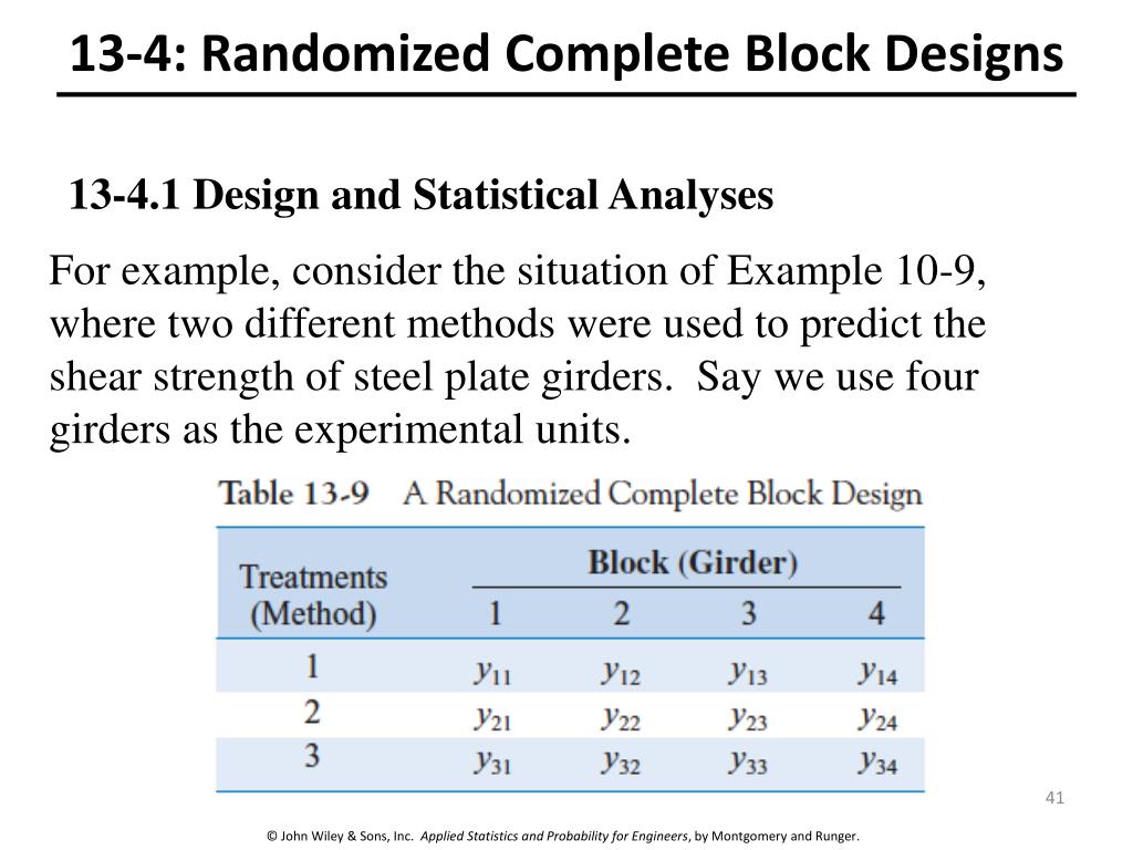
In this experiment, each specimen is called a “block”; thus, we have designed a more homogenous set of experimental units on which to test the tips. This kind of design is used to minimize the effects of systematic error. If the experimenter focuses exclusively on the differences between treatments, the effects due to variations between the different blocks should be eliminated. In this case, we would have four rows, one for each of the four varieties of rice. In this case, we have five columns, one for each of the five blocks.
Randomized Complete Block Design Analysis Model
Days of the week are not all the same, Monday is not always the best day of the week! Just like any other factor not included in the design you hope it is not important or you would have included it into the experiment in the first place. For instance, we might do this experiment all in the same factory using the same machines and the same operators for these machines.
Statistical Analysis of the Latin Square Design
In case all samples cannot be processed together, one first createsthe batches, and subsequently performs block randomization withineach batch. For example, say we have to process the above samplesin two batches. Given that we are interested in all comparisons betweenthe treatment–sex combinations, we make two batches of 12 samples,each batch containing three subjects of each group (Figure Figure55). This way, the batches arebalanced in terms of the subject-characteristics that we use in theanalytical model. Here we have two pairs occurring together 2 times and the other four pairs occurring together 0 times.
When should you use blocking?
Table 2 : Efficiency of RBD in comparison to CRD when plots were... - ResearchGate
Table 2 : Efficiency of RBD in comparison to CRD when plots were....
Posted: Fri, 08 Jun 2018 16:57:07 GMT [source]
The smallest crossover design which allows you to have each treatment occurring in each period would be a single Latin square. The previous examples includedtwo groups of subjects where thetreatment was assumed to be the only difference, and where all samplescould be processed at the same time. Most experiments have to accountfor control variables when estimating the treatment effects.
Here is an actual data example for a design balanced for carryover effects. In this example the subjects are cows and the treatments are the diets provided for the cows. Using the two Latin squares we have three diets A, B, and C that are given to 6 different cows during three different time periods of six weeks each, after which the weight of the milk production was measured. To compare the results from the RCBD, we take a look at the table below. What we did here was use the one-way analysis of variance instead of the two-way to illustrate what might have occurred if we had not blocked, if we had ignored the variation due to the different specimens.
Significance Level

If this point is missing we can substitute x, calculate the sum of squares residuals, and solve for x which minimizes the error and gives us a point based on all the other data and the two-way model. We sometimes call this an imputed point, where you use the least squares approach to estimate this missing data point. Another way to look at these residuals is to plot the residuals against the two factors. Notice that pressure is the treatment factor and batch is the block factor.
The first replicate would occur during the first week, the second replicate would occur during the second week, etc. Week one would be replication one, week two would be replication two and week three would be replication three. We now illustrate the GLM analysis based on the missing data situation - one observation missing (Batch 4, pressure 2 data point removed). The least squares means as you can see (below) are slightly different, for pressure 8700. What you also want to notice is the standard error of these means, i.e., the S.E., for the second treatment is slightly larger.
This means that we only observe every treatment once in eachblock. Imagine an extreme scenario where all of the athletes that are running on turf fields get allocated into one group and all of the athletes that are running on grass fields are allocated into the other group. In this case it would be near impossible to separate the impact that the type of cleats has on the run times from the impact that the type of field has. Identify potential factors that are not the primary focus of the study but could introduce variability. Connect and share knowledge within a single location that is structured and easy to search.
Lowering the thermal noise barrier in functional brain mapping with magnetic resonance imaging - Nature.com
Lowering the thermal noise barrier in functional brain mapping with magnetic resonance imaging.
Posted: Mon, 30 Aug 2021 07:00:00 GMT [source]
For a complete block design, we would have each treatment occurring one time within each block, so all entries in this matrix would be 1's. For an incomplete block design, the incidence matrix would be 0's and 1's simply indicating whether or not that treatment occurs in that block. The choice of case depends on how you need to conduct the experiment. If you are simply replicating the experiment with the same row and column levels, you are in Case 1. If you are changing one or the other of the row or column factors, using different machines or operators, then you are in Case 2. If both of the block factors have levels that differ across the replicates, then you are in Case 3.
First, the blocking variable should have an effect on the dependent variable. Just like in the example above, driving experience has an impact on driving ability. This is why we picked this particular variable as the blocking variable in the first place.
I think most of the time it’s just a matter of convention, likely proper to each field. I think that in medical context, in a two factors anova one of the factors is almost always called "treatment" and the other "block". Note that the least squares means for treatments when using PROC Mixed, correspond to the combined intra- and inter-block estimates of the treatment effects.


No comments:
Post a Comment